.jpg)
Introduction
This report shows the results of a test survey aimed at comparing four different UAV-based (Unmanned Aerial Vehicle) magnetometers and their capabilities to detect various infrastructure utilities.
The test was carried out on the 20-21st of September 2023 in the SPH Engineering UAV test range in Baloži, Latvia (N 56.8631°, E 24.1119°), in which dozens of various ferrous (magnetic) and non-ferrous material utilities are buried in different depths. Target detection and data processing were done using Seequent Oasis Montaj software. The devices used in this test were MagNIMBUS by SPH Engineering, MagDRONE R3 by SENSYS, MagArrow II by Geometrics, and DRONEmag GSMP-35U by GEM Systems.
Data collected by Sergejs Kucenko1. Data processing and report by Matīss Brants1.
1 SPH Engineering SIA, Latvia
Disclaimer:
" detected " means that the data interpreter has identified a strong enough signal that warrants further examination or action. Interpretations are subjective and will change depending on the experience and knowledge of the interpreter.
Neither SPH Engineering SIA, SENSYS Sensorik & Systemtechnologie GmbH, Geometrics Inc., nor GEM Systems Inc. makes any claims or warranty that detection of the same or similar or similar targets is guaranteed under any conditions other than in the SPH Engineering test range using the same or different hardware, software and workflow.
This report is provided "as is" and is intended to demonstrate the capabilities of the system described herein and provide some guidance for planning utility detection surveys.
Methods
The test setup
The test was conducted at the "SPH Engineering SIA" UAV test range in Baloži, Latvia, a 4-hectare large, open field surrounded by forests in a relatively magnetically quiet area. 23 objects that simulate underground utilities, like steel pipes and barrels, are buried. The ferrous (magnetic) targets detected with magnetometer technology are listed in Table 1, while their relative positions can be viewed in Figure 1. Objects made of other metals, i.e., aluminum, copper, gold, etc., cannot be detected, apart from special cases where the objects carry an electric current.
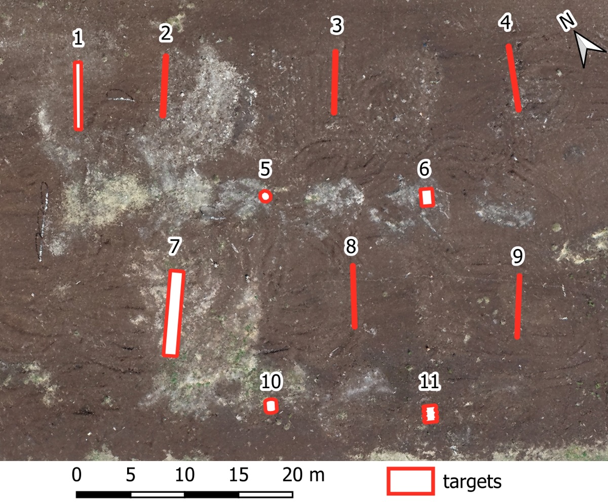
Table 1. Ferrous (magnetic) buried objects in the test range.
Each drone was flown in parallel lines with approximately 1.0-meter separation over the test range at a constant sensor altitude of 1.0 meters. This means that while the magnetometers were 1.0 m above the ground level, the drone was at a higher altitude, depending on the setup. The flight lines were planned with a sufficient run-off at the ends to account for different setup requirements for steady and controlled flights. All flights were conducted by an experienced UAV pilot on a pre-planned route using the SPH Engineering UgCS (Universal Ground Control System) software and SkyHub onboard computer. A True-Terrain Following system developed by SPH Engineering was used for precise altitude determination.
Magnetometers
All magnetometers were attached to a DJI Matrice 300 RTK UAV, which utilized GNSS (Global Navigation Satellite System) with RTK (Real Time Kinematics) for precise positioning. For geotagging, a different approach was used for different magnetometers:
- MagNIMBUS: Data logging is on SkyHub onboard computer using coordinates streamed from the drone’s GNSS receiver, which was in RTK mode during the tests.
- MagDrone R3: that magnetometer has an internal data recorder, but the coordinates stream was supplied from the drone’s GNSS receiver through the SkyHub onboard computer.
- MagArrow Mk2 has an internal data logger and internal RTK GNSS receiver, but it was in non-RTK mode during the tests. After the flight coordinates in the data were replaced with precise coordinates from the flight log, recorded by SkyHub (the drone was in RTK mode).
- DRONEmag GSMP-35U has an internal data recorder, and a separate GNSS receiver was connected directly to the recorder. That GNSS receiver was in non-RTK mode, and coordinates in logged data were refined using flight track recorded by SkyHub.
SPH Engineering's True Terrain Following system (TTF) ensured precise altitude above the ground.
MagNIMBUS
The SPH Engineering manufactured MagNIMBUS system (figure 2) utilizes a QuSpin Total-Field Magnetometer placed at the end of a collapsible "arm" under the UAV, which protects the system from damage in case of a collision with unexpected obstacles and permits extremely low flights with relative safety. The QuSpin sensor records total magnetic intensity at a rate of 500 Hz, which allows it to filter out any magnetic noise picked up from electrical parts of the UAV and nearby alternating electromagnetic sources like power lines. The setup was flown at a constant speed of 3 m/s.
MagDrone R3
The MagDrone R3 by SENSYS GmbH is a magnetometer system (figure 3) with two 3-axis fluxgate vectorial sensors built into the ends of a one-meter-long tube. This dual-sensor setup reduces flight time by at least 50% compared to single-sensor setups. The device is attached directly to the legs of the UAV, thus providing stable and relatively predictable sensor movement while also placing the magnetometers closer to the magnetic interference of the motors of the UAV. Both sensors record the magnetic field in all three axes at a sampling rate of 250 Hz to allow the removal of the alternating noise of UAV motors and other sources like power lines. The setup was flown at a constant speed of 2 m/s.
MagArrow II
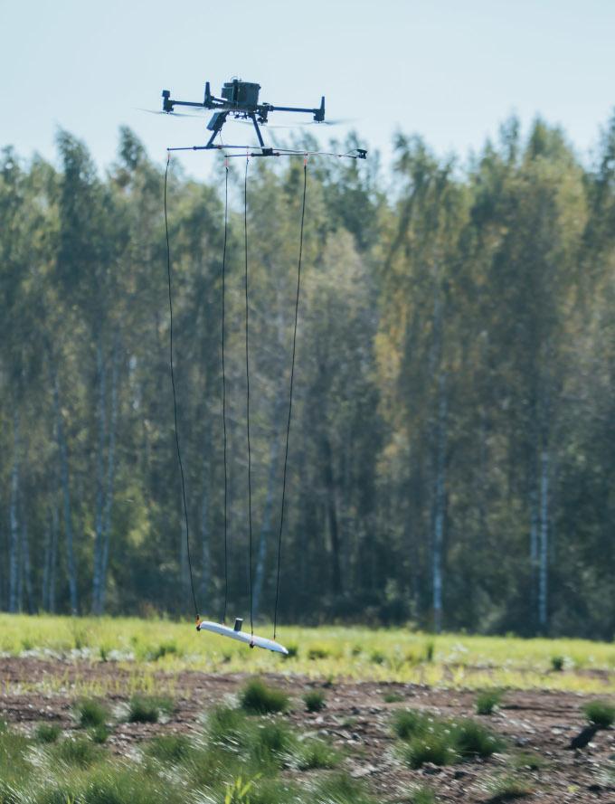
The Geometrics MagArrow II magnetometer (figure 4) utilizes a wire-suspended setup in an aerodynamic enclosure to place the total field magnetometer sensor as far away from the interference of the UAV as possible. Even with such a placement, the very high sampling rate of 1000 Hz allows for filtering out any remaining alternating magnetic noise caused by the UAV or other sources like power lines. The suspended setup increases the movement of the magnetometer encasement, causing magnetic field reading changes. Thus, a heading calibration flight is highly recommended.
For this test, the MagArrow II magnetometer was suspended in a 3-meter-long cable system, and the flight was done at a constant UAV speed of 3 m/s.
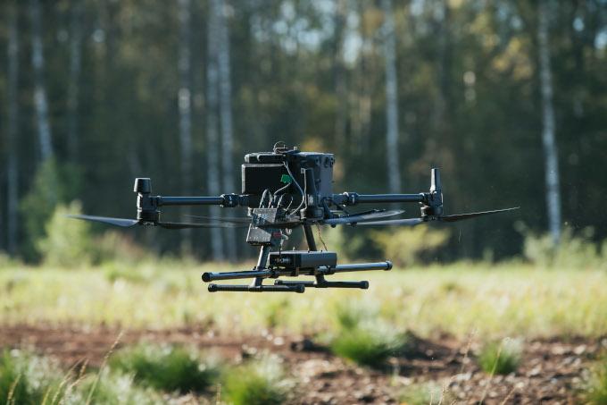
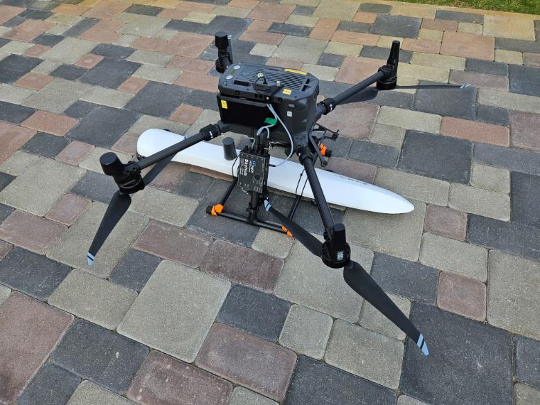
Also, a second test was done with MagArrow II attached directly to drone legs (figure 5) instead of using the suspension system. In this case, the flight speed was also 3 m/s.
DRONEmag GSMP-35U
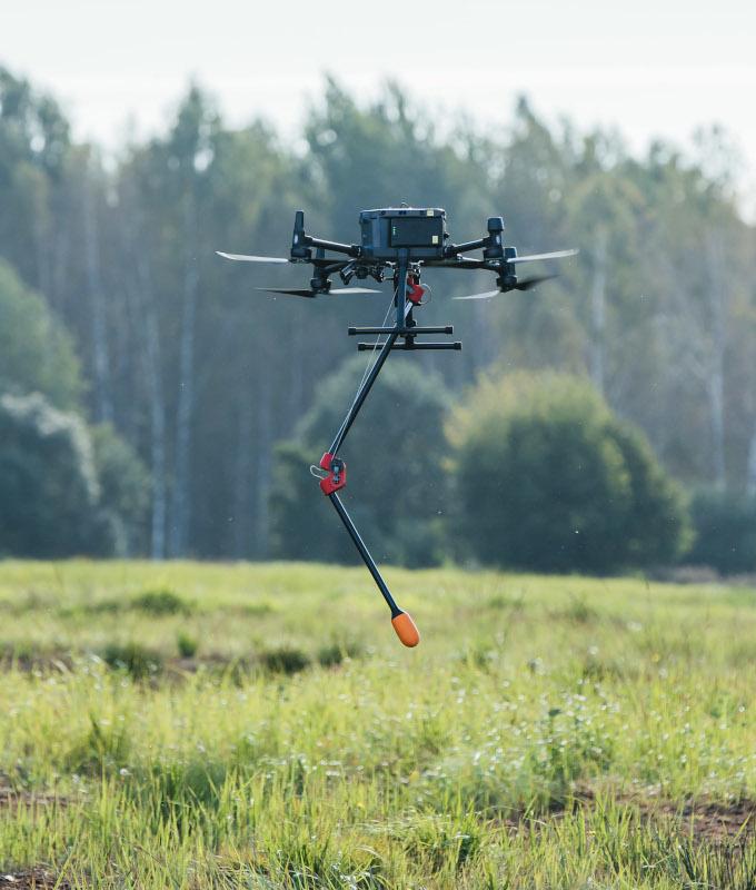
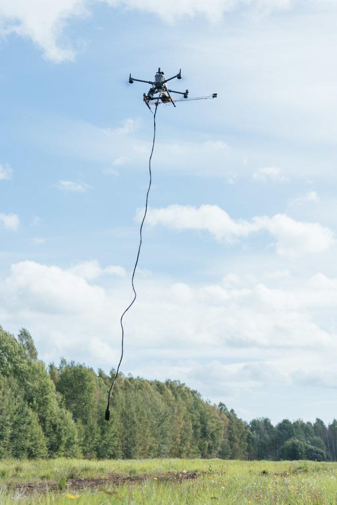
The GEM Systems DRONEmag GSMP-35U is a total-field magnetometer system (figure 6) suspended in a 3-5 m cable from the UAV. This setup provides maximum distance from the magnetic interference of the UAV's motors. Such a setup allows for a much lower sampling rate of a maximum of 20 Hz than the manufacturers' sensors. A low sampling rate also provides easier and faster data processing. The setup was suspended in a 5-meter-long cable and flown at a constant UAV speed of 3 m/s.
Data processing
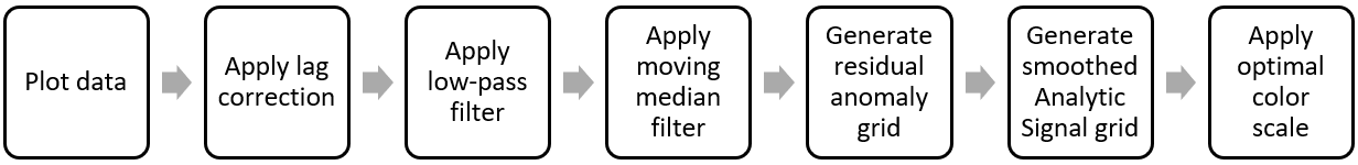
Magnetic data processing was done as similarly as possible for all systems, except for specific data format conversions for MagDRONE R3 and MagArrow II systems, which required proprietary software. The general workflow is outlined in Figure 7, with a detailed step-by-step account for all setups in the Appendix. The main software used was Geosoft Oasis Montaj Standard Edition v.2023.1. utilizing only the base module features and well-documented processing methods. All the steps may be repeated with similar results using closed and open-source software.
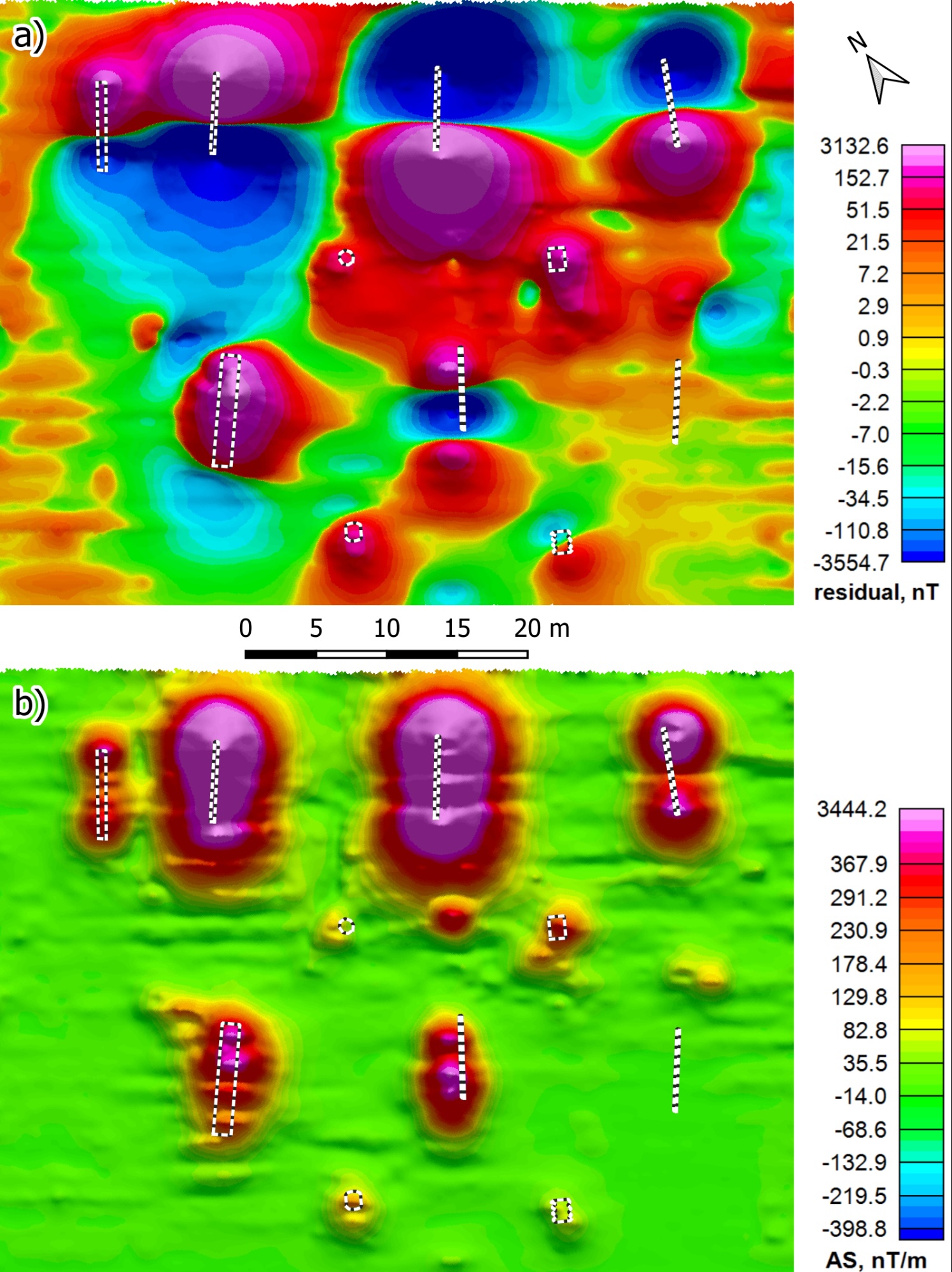
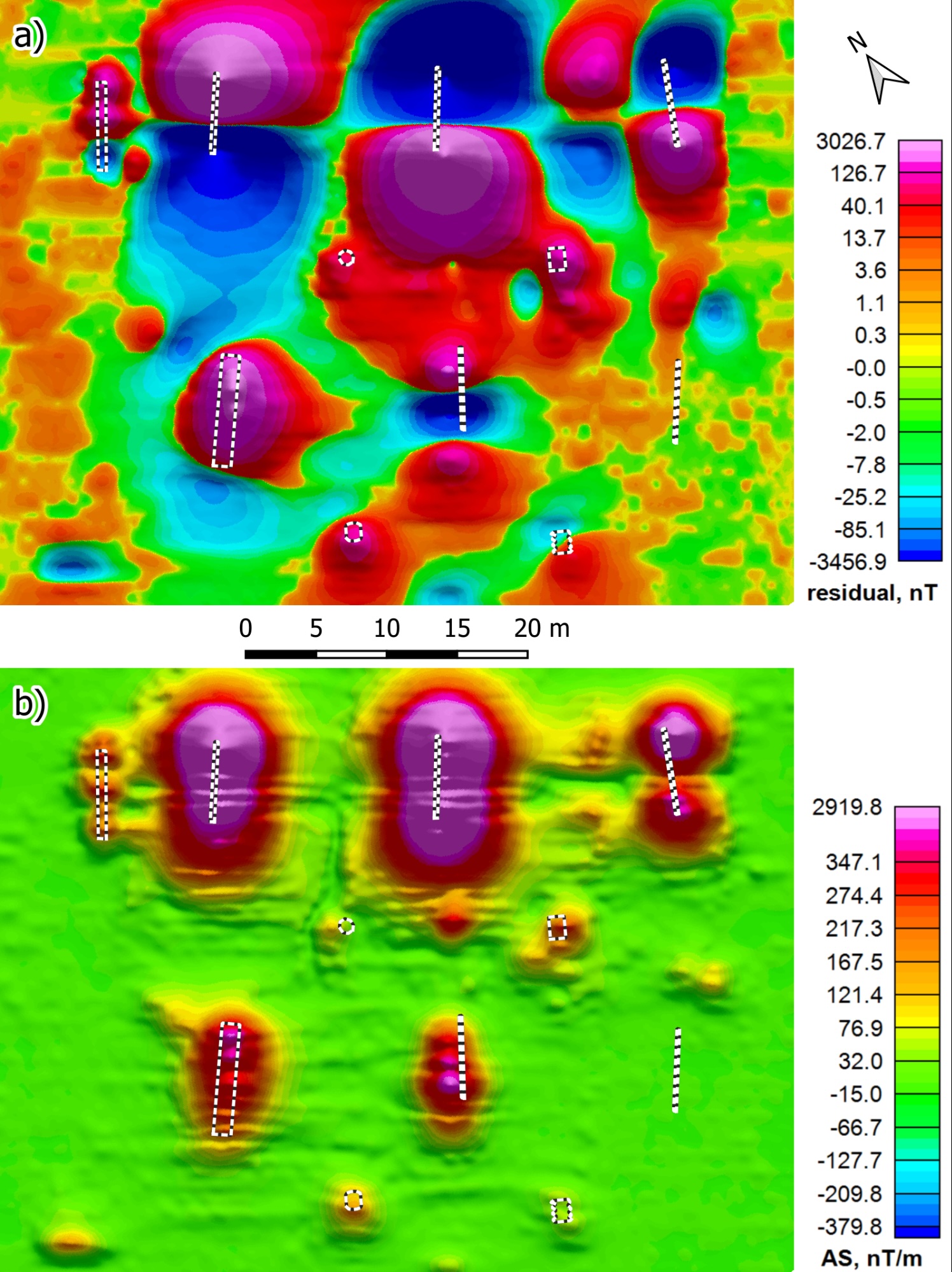
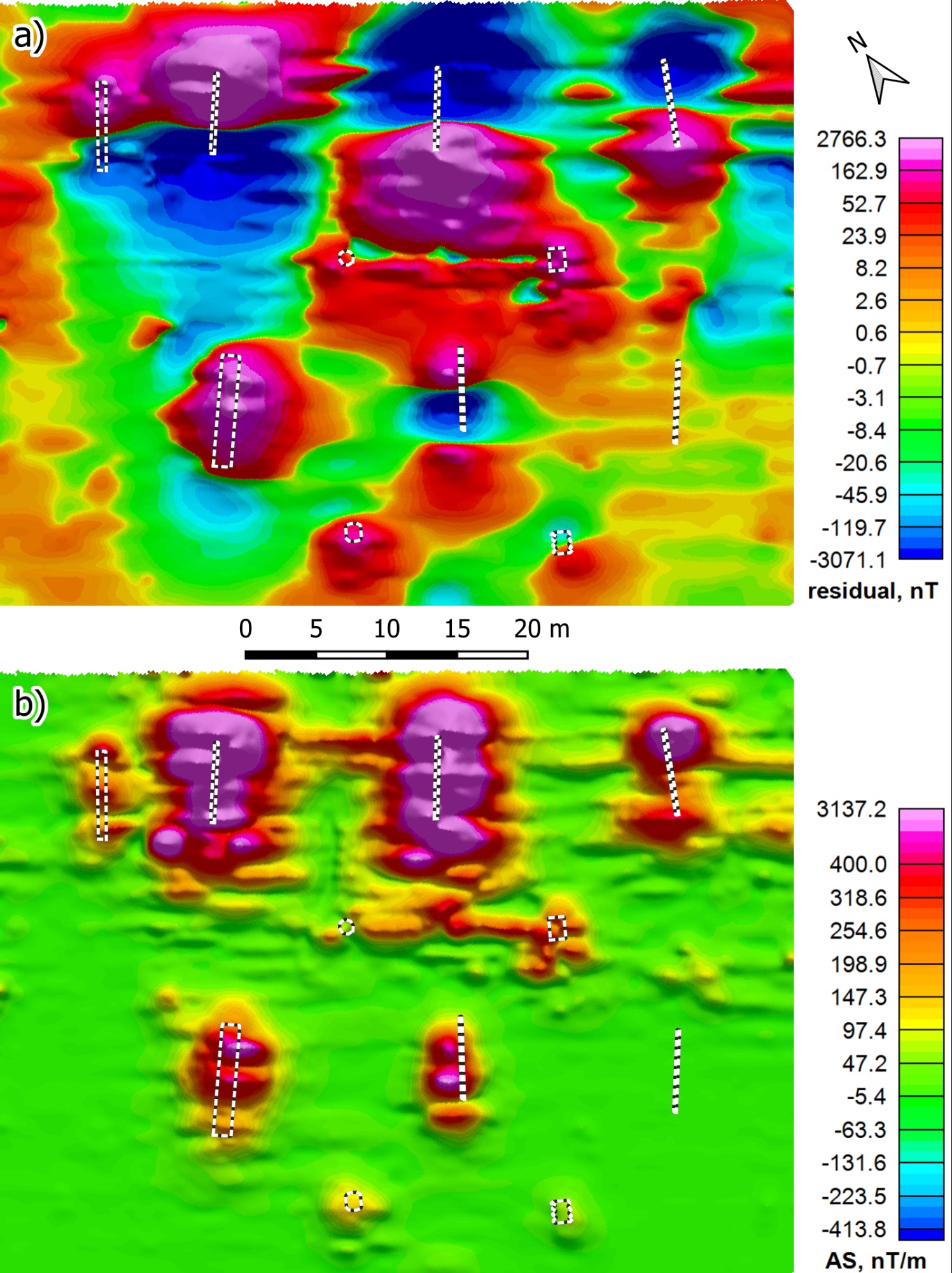
The processed data was visualized as residual anomalous magnetic field grids and its Analytic Signal (AS). A cell size of 0.2 meters was chosen to account for the very dense in-line sampling points and the relatively sparse separation of flight lines of 1.0 meters. This helps retain the high resolution in a direction parallel to the flight path while providing a smoother grid perpendicular to the lines. Shading, which simulates relief, was applied for all grids to enhance the visualization of smaller anomalies.
Results
All sensors appear to have detected all the test targets but one – no. 9 steel pipe with a 1.5mm wall, which is likely due to the relatively thin walls of the object. In all other cases, the main difference between the sensors lies in the clarity of the detected signals and the amount of signal noise. The most important noise source is heading error, caused by magnetic interference from the sensor system setup and is visible as "streaks" in the direction of flight, especially in the analytic signal maps. This is enhanced on suspended systems, which are more prone to wind and weight over-loading. A strong magnetic anomaly was also detected by all sensors near target no.3, which was an unidentified iron scrap and is ignored in this survey.
SPH Engineering's MagNIMBUS data (figure 8) show a good resolution of the target magnetic anomalies with well-defined borders. Only some noise streaking is visible, but it does not interfere with target signals.
SENSYS MagDrone R3 data (figure 9) also show well-defined, compact anomalies. The streaking is quite noticeable in the target signals but does not decrease the detection quality. The background looks quite noise-less. Of importance are the false positive anomalies between targets 3 and 4 (upper-right corner) in the residual anomaly map and, to a lesser extent, also the analytic signal map. This data processing artifact occurs when a moving median filter is used on separated data lines.
Geometrics MagArrow II suspended setup data (figure 10) also show well-developed anomaly signals; all targets are visible. Some noticeable streaking between anomalies also disturbs the signals, but the background is fairly noise-less. Although heading error correction was applied to data, the suspended setup still causes notable streaking, which more advanced data processing techniques could eliminate.
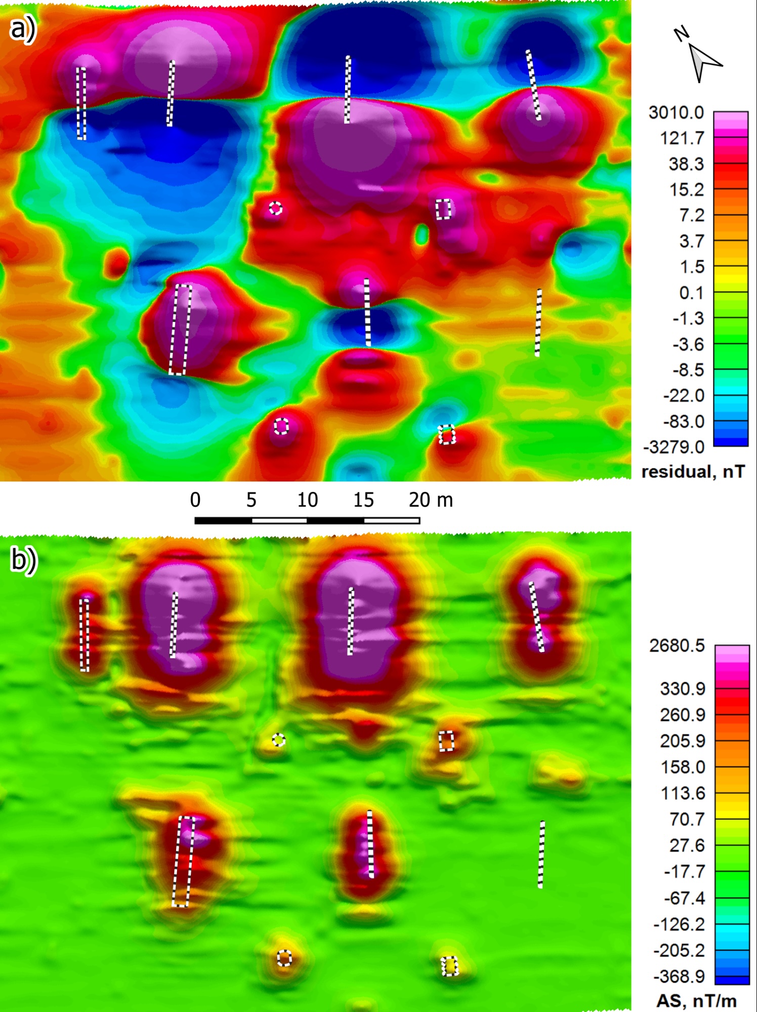
The same Geometrics MagArrow II sensor in a fixed setup fared surprisingly well despite the sensor being close to drone motors. The maps (figure 11) show noticeable streaking, which is tolerable, yet the anomalies are well-defined and arguably better than in the suspended setup data.
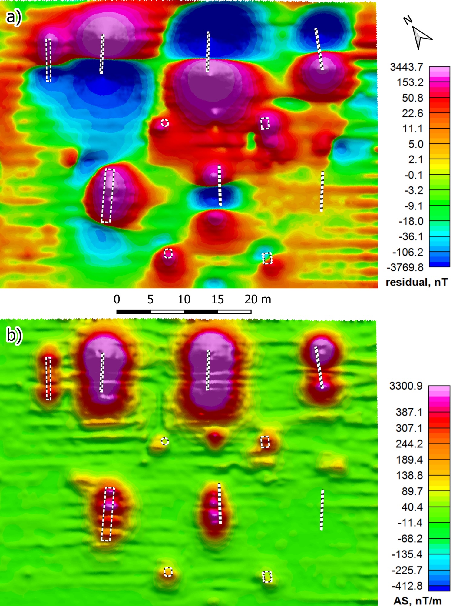
GEM Systems GSMP-35U data (figure 12) is quite noisy, with chaotic streaking and disfigured anomaly boundaries. Yet the background is almost noise-less, and the anomalies are still clearly distinguishable for the most part. The cause of the magnetic data distortions might be the heavy weight of the setup, which overloaded the drone, while moderate side winds enhanced the effect. The chosen low sampling rate of 20 measurements per second also hindered data processing at times – it should be preferably set to at least 40 measurements per second.
Conclusions
- All sensors detected 10 out of 11 magnetic targets in the test range.
- MagNIMBUS yielded arguably the best results with low noise and well-defined target signals.
- The MagDrone R3 showed slightly more noisy data but still a very good resolution of anomalies, although noteworthy data processing artifact issues exist.
- MagArrow II was tested in two setups: the fixed setup proved to be arguably better than the suspended setup in resolving target anomalies, but the results were very good in both cases.
- GSMP-35U fared the worst with quite noticeable noise and distorted anomaly boundaries, although the cause was the overloaded weight of the setup and windy conditions.
- This comparison hints that the magnetometer sensor sensitivities are already very respectable, but the shortcomings of setups hinder the acquisition of high-quality data. The main problem for the suspended setups is the overloading of the DJI M300 drone, especially in more windy conditions. The fixed setups with a high sampling rate in this test provided the best results.
Appendix - data processing steps
MagNIMBUS
Using Oasis Montaj:
1. Applied Lag Correction of -130 fiducials;
2. Applied low-pass filter of 100 fiducials (corresponding to ~0.2 m point separation);
3. Applied Rolling median of 10000 fiducials (corresponding to 60 m);
4. Generated residual anomaly grid with cell size 0.2 m, color scale Histogram equalization;
5. Calculated Analytic Signal based on residual anomaly grid;
6. Applied 3x3 convolution 1 pass smoothing to the AS grid and changed the color scale to Normal distribution.
MagDRONE R3
1. Using MagDrone DataTool:
1.1. Imported file 20230920_063633_MD-R3_#0207.mdd
1.2. Divided into tracks.
1.3. No filters or downsampling.
1.4. Loaded GNSS RTK data.
1.5. Exported to .asc file.
2. Using Oasis Montaj:
2.1. Divided lines based on sensor ID;
2.2. Separated each flight in lines by sensor number;
2.3. Corrected time lag: -30 fiducials;
2.4. Applied Low Pass Filter of 25 fiducials (corresponding to ~0.2 m point separation).
2.5. Applied Rolling Median filter of 7500 fiducials (corresponding to ~60 m distance).
2.6. Generated residual anomaly grid with cell size 0.2 m and calculated Analytic Signal.
2.7. Applied 3x3 convolution 1 pass smoothing to the AS grid and changed the color scale to Normal distribution
MagArrow II (suspended setup)
Using Geometrics Survey Manager:
1. Data converted from MagArrow .magdata to .csv data format.
Using Oasis Montaj:
1. Applied Heading correction with data acquired on calibration flight.
2. Applied Lag Correction of +100 fiducials
3. Applied low-pass filter of 67 fiducials (corresponding to ~0.2 m point separation).
4. Applied Rolling Median filter of 20000 fiducials (corresponding to ~60 m window).
5. Generated residual anomaly grid with cell size 0.2 m, color scale Histogram equalization.
6. Calculated Analytic Signal.
7. Applied 3x3 convolution 1 pass smoothing to the AS grid and changed the color scale to Normal distribution.
MagArrow II (fixed setup)
Using Geometrics Survey Manager:
1. Data converted from MagArrow .magdata to .csv data format.
Using Oasis Montaj:
1. Applied Heading correction with data acquired on calibration flight.
2. Applied Lag Correction of +300 fiducials
3. Applied low-pass filter of 67 fiducials (corresponding to ~0.2 m point separation).
4. Applied Rolling Median filter of 20000 fiducials (corresponding to ~60 m window).
5. Generated residual anomaly grid with cell size 0.2 m, color scale Histogram equalization.
6. Calculated Analytic Signal.
7. Applied 3x3 convolution 1 pass smoothing to the AS grid and changed the color scale to Normal distribution.
GSMP-35U
Using Oasis Montaj:
1. Imported GNSS coordinates into mag database;
2. Applied Lag Correction (variable):
- Flight no.1 from 08:27:37 till 08:35:20: +6
- Flight no.1 from 08:35:20 till 08:38:43 +8
- Flight no.2: +4
- Flight no.3: +7
3. Applied low-pass filter of 2 fiducials (corresponding to ~0.2 m point separation).
4. Applied Rolling Median filter of 400 fiducials (corresponding to ~60 m window).
5. Generated residual anomaly grid with cell size 0.2 m, color scale Histogram equalization.
6. Calculated Analytic Signal.
7. Applied 3x3 convolution 1 pass smoothing to the AS grid and changed the color scale to Normal distribution.