The test was carried out on the 21st of September, 2023, at the SPH Engineering UAV test site in Baloži, Latvia (N 56.8631°, E 24.1119°). Three UXO-like objects were placed on the field, conforming to the ISO SEEDS standard, with magnetic characteristics analogous to 20-, 60-, and 105-mm shells. During the test, magnetometers attached to a UAV were flown over the test targets at different altitudes. Target detection was done in software after data processing. The devices used in this test were MagNIMBUS by SPH Engineering, MagDrone R3 by SENSYS, MagArrow II by Geometrics, and DRONEmag GSMP-35U by GEM Systems.
Data collected by Sergejs Kucenko1. Data processing and report by Matīss Brants1.
1 SPH Engineering SIA, Latvia
Disclaimer
The term "detected" here means that the data interpreter has identified a strong enough signal that warrants further examination or action. Interpretations are subjective and will change depending on the experience and knowledge of the interpreter.
Neither SPH Engineering SIA, SENSYS Sensorik & Systemtechnologie GmbH, Geometrics Inc., nor GEM Systems Inc. makes any claims or warranty that detection of the same or similar or similar targets is guaranteed under any conditions other than in the SPH Engineering test range using the same or different hardware, software, and workflow.
This report is provided "as is" and is intended to demonstrate the capabilities of the system described herein and provide some guidance for planning UXO surveys.
Methods
The test setup
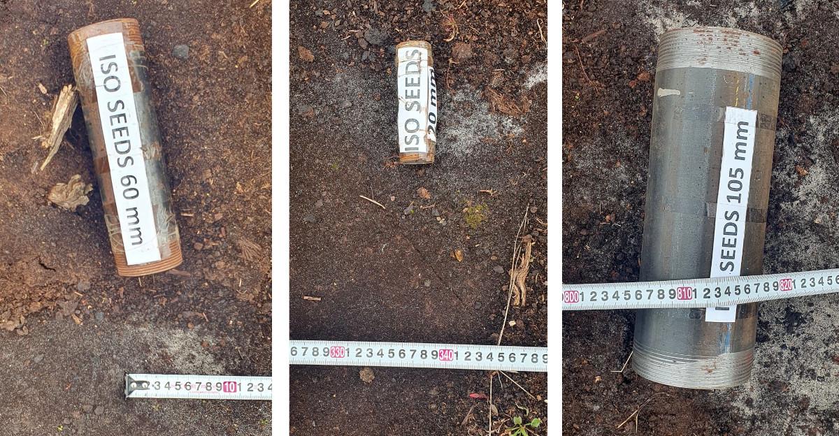
The test was conducted at the "SPH Engineering SIA" UAV test site in Baloži, Latvia, a 4-hectare large, open field surrounded by forests in a magnetically relatively quiet area. The UXO test setup comprises three different, standardized ISO SEEDS objects placed along an 8-meter-long profile with their longest axis in a SW-NE direction. The ISO SEEDS objects were analogous to 60 mm, 20 mm, and 105 mm ordnance shells (figure 1). For simplicity, in the further text, these objects will be referred to as "ordnance," "shell," or "UXO." The test area could be defined as non-magnetic, consisting of mainly reworked peat, although some small anthropogenic magnetic objects were identified nearby and are visible in the visualized results.
Each magnetometer setup was flown in parallel lines over the UXO objects and the surrounding area during the test. After each successful pass, the altitude was raised, starting from 0.5 meters to 2.5 meters above ground level in 0.5-meter increments, thus surveying the test area 5 times. It must be stressed that the different flight altitudes in this test simulate the distance from the magnetometer to the UXO, not the magnetometer's height above ground level. For example, the 2.5-meter flight test results predict the detection capabilities of a sensor as if it was flown 0.5 meters above the ground and a UXO at a depth of 2.0 meters was buried underground.
The flight lines were planned with a 10-meter run-off at the ends to account for different setup requirements for steady and controlled flights. All flights were conducted by an experienced UAV pilot on a pre-planned route using the SPH Engineering UgCS (Universal Ground Control System) software and SkyHub onboard computer. A True-Terrain Following system developed by SPH Engineering was used for precise altitude determination.
Magnetometers
All magnetometers were attached to a DJI Matrice 300 RTK UAV, which utilized GNSS (Global Navigation Satellite System) with RTK (Real Time Kinematics) for precise positioning. For geotagging, it was used a different approach for different magnetometers:
- MagNIMBUS: Data logging is on SkyHub onboard computer using coordinates streamed from the drone’s GNSS receiver, which was in RTK mode during the tests.
- MagDrone R3: that magnetometer has an internal data recorder, but the coordinates stream was supplied from the drone’s GNSS receiver through the SkyHub onboard computer.
- MagArrow Mk2 has an internal data logger and internal RTK GNSS receiver, but it was in non-RTK mode during the tests. After the flight coordinates in the data were replaced with precise coordinates from the flight log, recorded by SkyHub (the drone was in RTK mode).
- DRONEmag GSMP-35U has an internal data recorder, and a separate GNSS receiver was connected directly to the recorder. That GNSS receiver was in non-RTK mode, and coordinates in logged data were refined using flight track recorded by SkyHub.
To ensure precise altitude above the ground, SPH Engineering's True Terrain Following system (TTF) was used (the importance of this is discussed more in the Discussion section).
MagNIMBUS
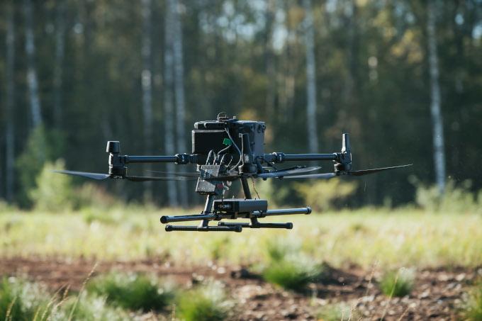
The SPH Engineering manufactured MagNIMBUS system (figure 2) utilizes a QuSpin Total-Field Magnetometer placed at the end of a collapsible "arm" under the UAV, which protects the system from damage in case of a collision with unexpected obstacles and permits extremely low flights with relative safety. The QuSpin sensor records total magnetic intensity at a rate of 500 Hz, which allows it to filter out any magnetic noise picked up from electrical parts of the UAV and nearby alternating electromagnetic sources like power lines. The setup was flown at a constant speed of 1 m/s.
MagDrone R3
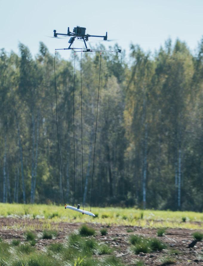
The MagDrone R3 by SENSYS GmbH is a magnetometer system (figure 3) with two 3-axis fluxgate vectorial sensors built into the ends of a one-meter-long tube. This dual-sensor setup reduces flight time by at least 50% compared to single-sensor setups. The device is attached directly to the legs of the UAV, thus providing stable and relatively predictable sensor movement while also placing the magnetometers closer to the magnetic interference of the motors of the UAV. Both sensors record the magnetic field in all three axes at a sampling rate of 250 Hz to allow the removal of the alternating noise of UAV motors and other sources like power lines. The setup was flown at a constant speed of 2 m/s.
MagArrow II
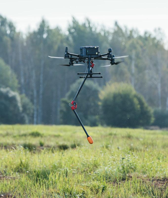
The Geometrics MagArrow II magnetometer (figure 4) utilizes a wire-suspended setup in an aerodynamic enclosure to place the total field magnetometer sensor as far away from the interference of the UAV as possible. Even with such a placement, the very high sampling rate of 1000 Hz allows for filtering out any remaining alternating magnetic noise caused by the UAV. The suspended setup increases the movement of the magnetometer encasement, causing magnetic field reading changes. Thus, a heading calibration flight is highly recommended. For this test, the MagArrow II magnetometer was suspended in a 3-meter-long cable system, and the flight was done at a constant UAV speed of 2 m/s.
DRONEmag GSMP-35U
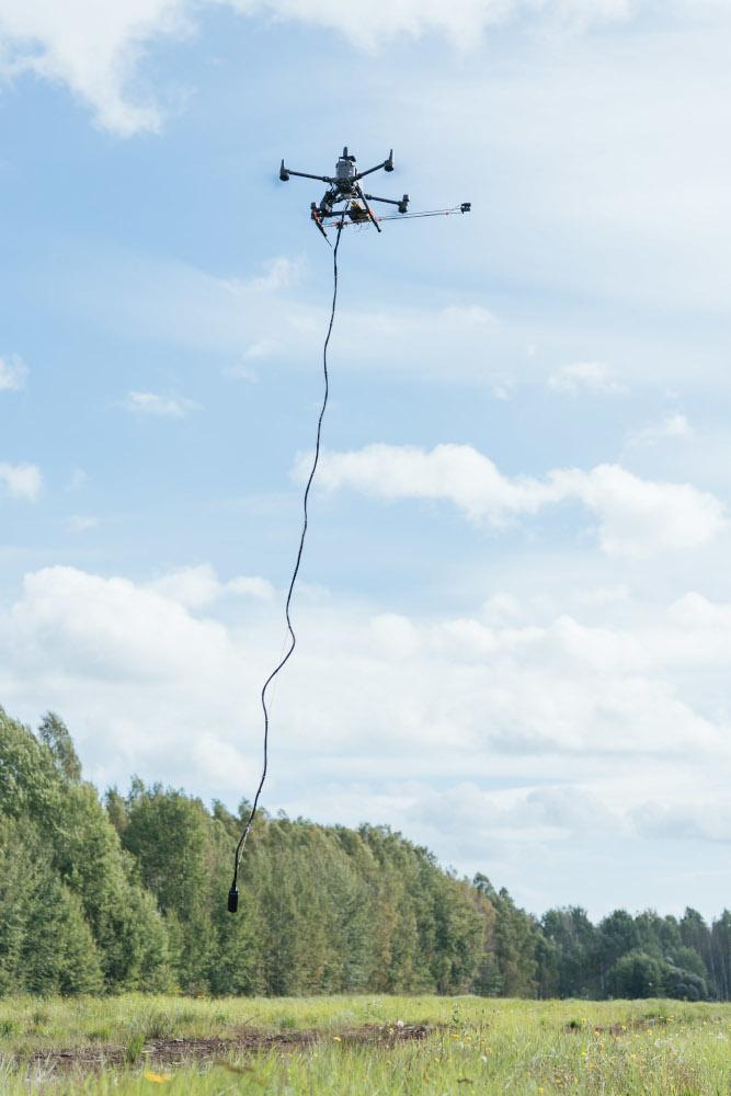
The GEM Systems DRONEmag GSMP-35U is a total-field magnetometer system (figure 5) suspended in a 3-5 m cable from the UAV. This setup provides maximum distance from the magnetic interference of the UAV's motors. Such a setup allows for a greatly lower sampling rate of a maximum of 20 Hz compared to other manufacturers' sensors. A low sampling rate also provides easier and faster data processing. The setup was suspended in a 5-meter-long cable and flown at a constant UAV speed of 1 m/s.
Data processing
Magnetic data processing was done for all systems as similarly as possible, except for specific data format conversions for MagDRONE R3 and MagArrow II systems, which required proprietary software. The general workflow is outlined in Figure 6, with a detailed step-by-step account for all setups in the Appendix. The main software used was Geosoft Oasis Montaj Standard Edition v.2023.1. utilizing only the base module features and well-documented processing methods. All the steps may be repeated with similar results using closed and open-source software.

Data visualization
Data visualization is a very important step in comparing the results of different devices, as it can be easily manipulated to create a bias toward a particular device. Thus, explaining the reasoning behind visualization techniques in detail was deemed necessary. Like data processing, a common approach was applied for all sensor data.
The processed data was visualized as residual anomalous magnetic field grids and its Analytic Signal (AS). A cell size of 0.2 meters was chosen to account for the very dense in-line sampling points and the relatively sparse separation of flight lines of 0.5 meters. This helps retain the high resolution in the direction parallel to the flight path while providing a smoother grid perpendicular to the lines. A shading, which simulates a relief, was applied for all grids to enhance the visualization of smaller anomalies.
Two grids were created for each flight pass and sensor:
1) residual anomalous field with a histogram-equalized color scale
and
2) analytic signal with a normally distributed color scale.
Although an AS grid with a histogram-equalized color scale better represents small anomalies, it also enhances the noise (figure 7).
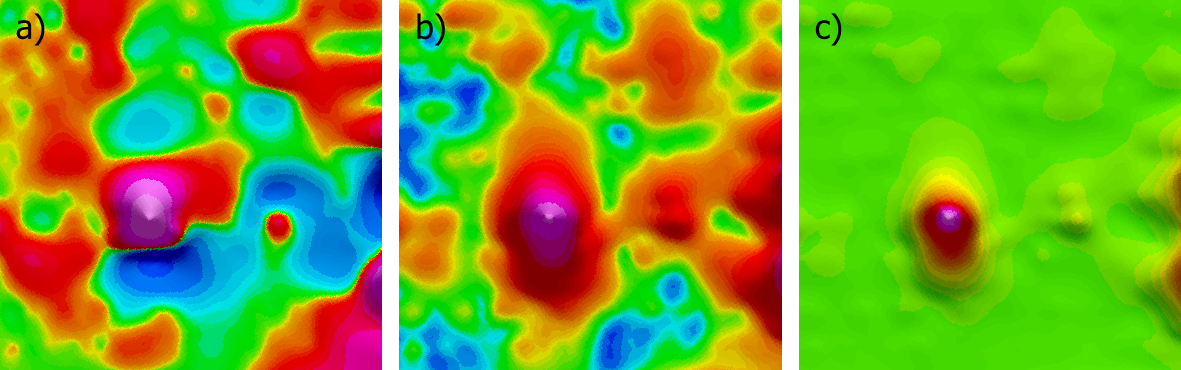
Ensuring fair representation is especially important at the lowest flight altitude when even slight changes in the trajectory over the target object will result in significant changes in magnetic field amplitudes. Applying the same values for the color scale would result in a bias towards some sensors. Due to this, the values of the grid color scale for each magnetometer were scaled automatically based on their own data amplitudes using the Color Tool in Oasis Montaj.
Results
Flight at 0.5 m altitude
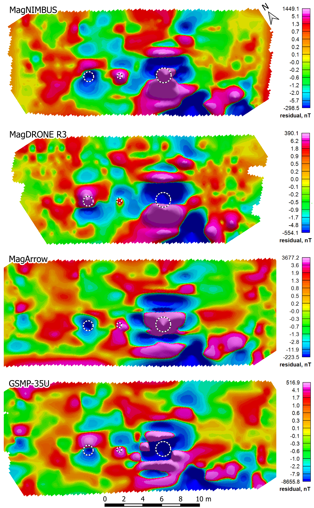
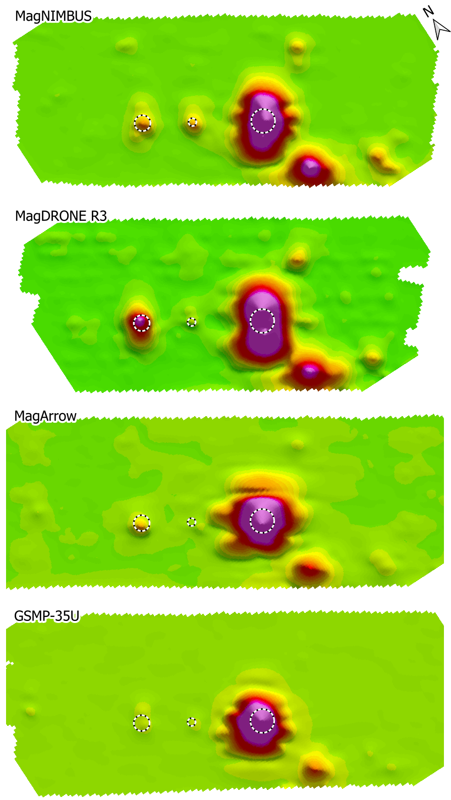
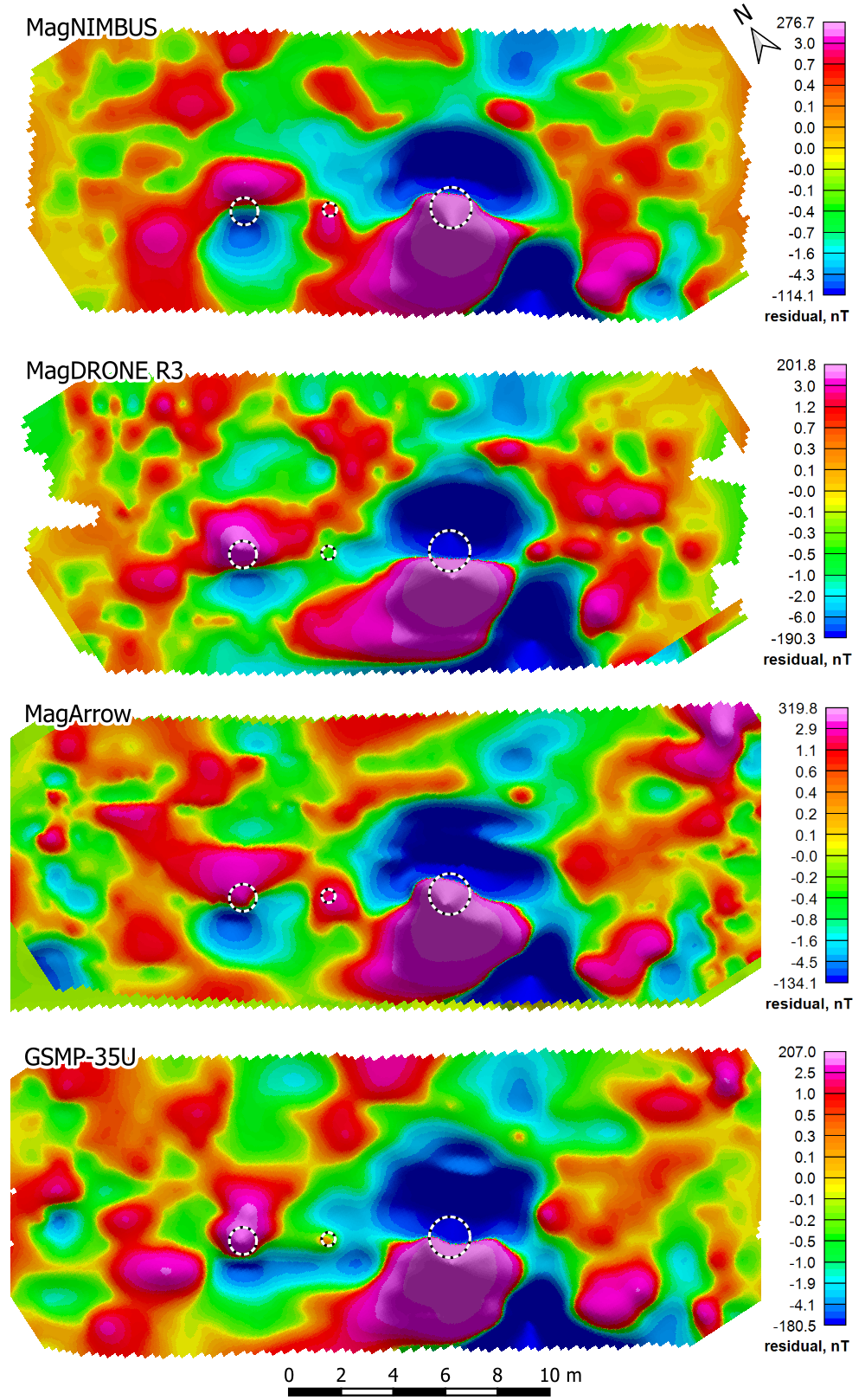
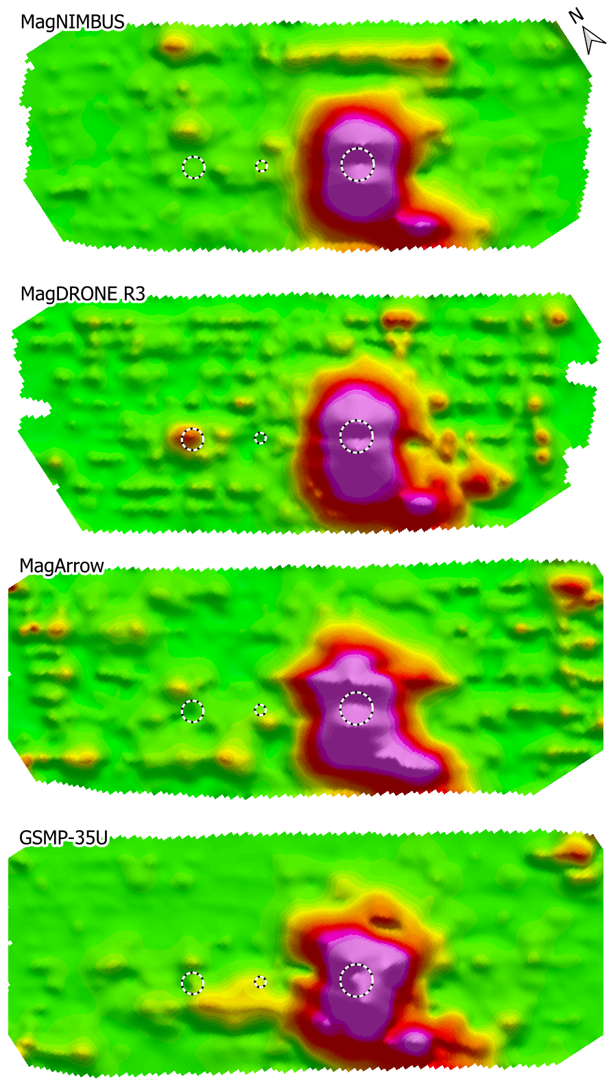
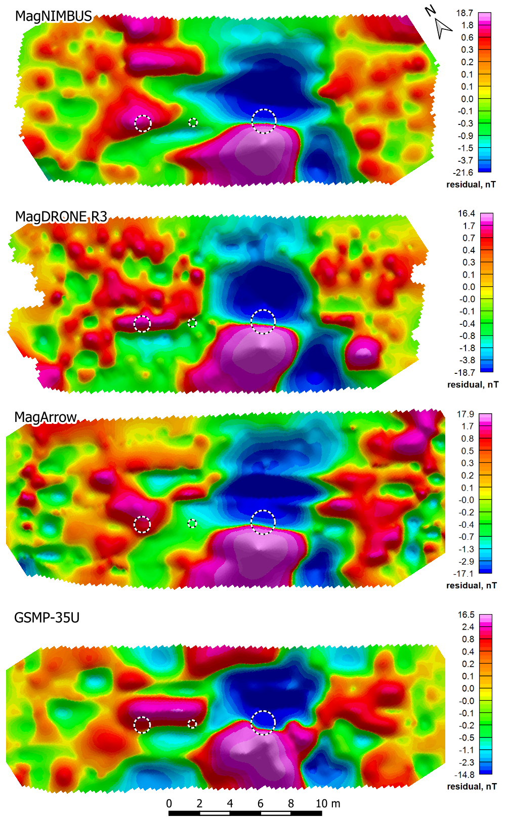
At an altitude of 0.5 meters above the targets, all sensors detected the smallest (20 mm shell) object to varying degrees. Still, the signal strength was very dependent on the trajectory of the sensor. The dipole in the residual anomaly grids (figure 8) is very pronounced in MagNIMBUS and GSMP-35U data, while for R3, the signal is weaker, although still unambiguous. In the case of MagArrow II, the dipole is close to unnoticeable, as the sensor passed mostly on the southern side of the object, although the signal would at least be considered suspicious. In all cases, the distorted dipole signals for the 105 mm shell are due to very high magnetic gradients.
The AS grids (figure 9) pinpoint the centers of the anomalies. MagNIMBUS clearly shows all anomalies, with the 60- and 20-mm shell anomalies being unexpectedly similar in size. The R3 magnetometer, however, shows a pronounced difference between the smaller anomalies. Both MagArrow II and GSMP-35U have a reduced signal for the smaller anomalies, but this is mostly due to the very high amplitude of the 105 mm shell anomaly - it distorts the color scale. This is why AS and residual anomalous field grids should always be inspected. The background noise is more pronounced in the R3 data, although still unmistakable. GEM System's GSMP-35U shows the "cleanest" background, most likely due to the 5m distance from the UAV.
Flight at 1.0 m altitude
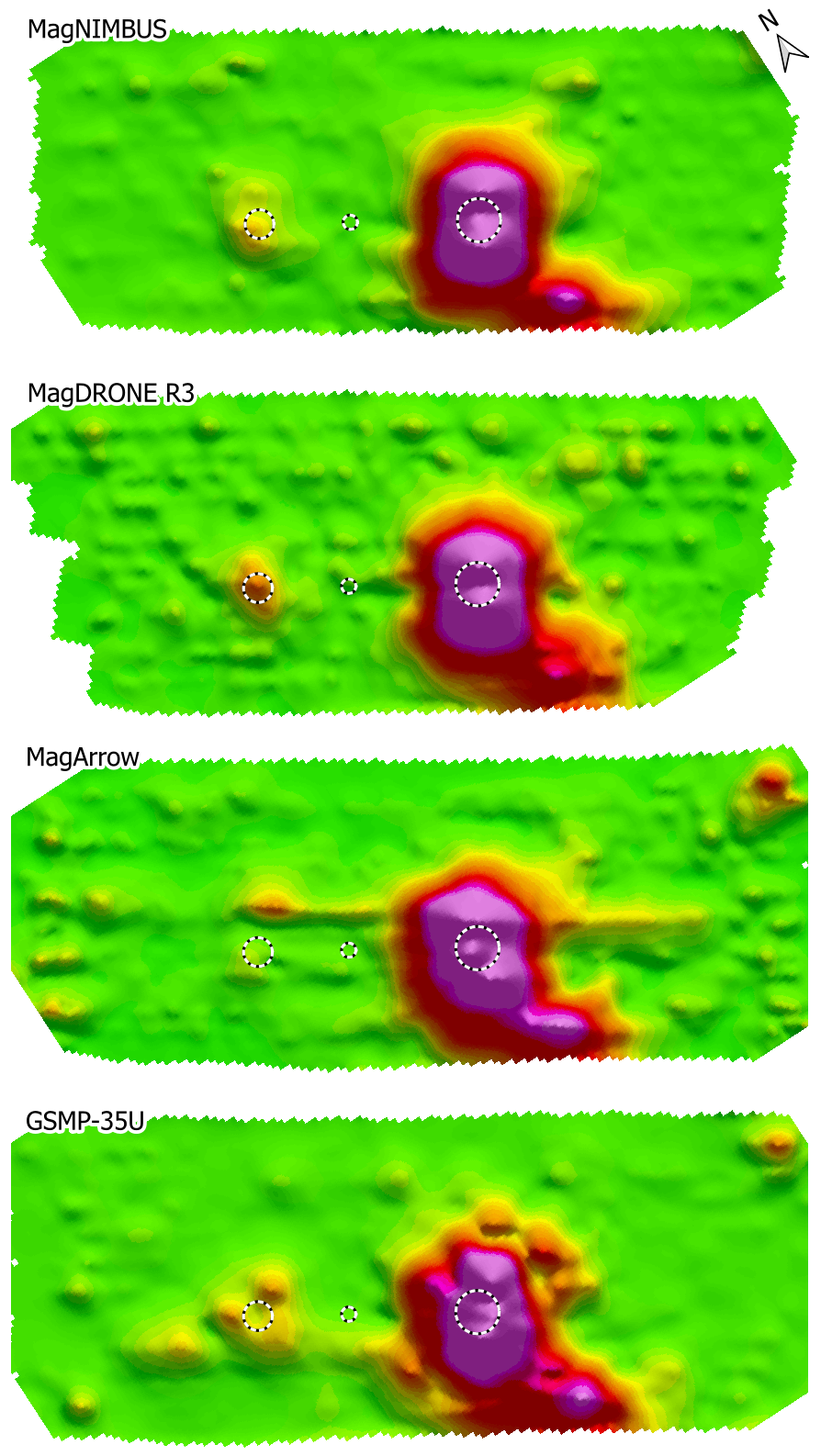
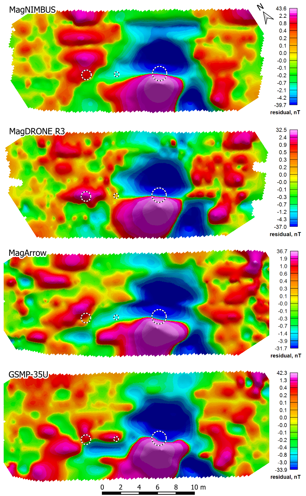
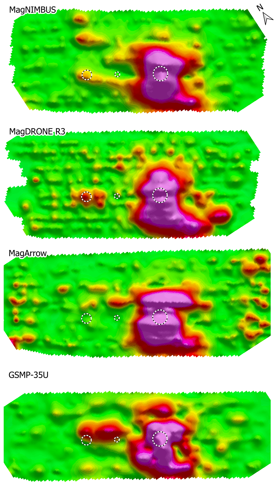
The 105 mm and 60 mm shell dipoles are clearly visible in the residual anomaly grids at 1.0 m flight altitude (figure 10). Due to lower magnetic gradients, the magnetic dipole of the 105 mm shell now also looks more "correct" in all cases. No sensor seems to have detected the 20 mm shell anymore. Although MagNIMBUS, MagArrow II, and GSMP-35U show a small anomaly near the location of the shell, it would probably be too similar to the noise to be considered a potential target.
AS grids also show no signs of a 20 mm shell signal (figure 11), but all sensors detected 60 mm and 105 mm shells. Although MagNIMBUS and MagArrow II show a less pronounced 60 mm shell signal, this seems to be due to flight trajectories nearly missing the target. Even so, the signal is clear in the residual anomaly grid. This time, the noise seems to be the lowest from the MagNIMBUS sensor, but all sensors start to show more random signals due to the decreasing signal-to-noise ratio.

Flight at 1.5 m altitude
At an altitude of 1.5 m, the sensors start to lose the signal of the 60 mm shell (figure 12). Meanwhile, for MagNIMBUS and R3, it is still a clear dipole signal. The GSMP-35U has experienced more noise, but MagArrow II suffers from unresolved heading errors despite heading correction. There are no signs of the 20 mm shell's signal for any of the sensors.
The AS grids reinforce these observations (figure 13). The R3 shows a distinct peak over the 60 mm shell's location, while for MagNIMBUS, it is more of a dispersed but still notable signal, but in the case of GSMP-35U, the signal seems somewhat distorted. However, it would definitely still attract attention in a real scenario. These strong signal peaks also seem to surround the anomaly of the 105 mm shell, but the cause of this is unknown. The heading errors of MagArrow II result in a long streak across most of the field and end with a stronger peak near the left-most anomaly, but this probably would not be considered a potential target.

Flight at 2.0 m altitude
At the distance of 2.0 m (figure 14), the 60 mm shell's anomaly loses the negative pole and turns into simply a positive magnetic anomaly. Of all the sensors, the R3 shows the most distinct signal, while for the rest of the sensors, the signal seems to be very close to the noise level and should not be counted as "detected." The AS grids (figure 15) generally show the same trends.
Flight at 2.5 m altitude
At the highest altitude of 2.5 meters, the residual anomaly grids (figure 16) for all sensors still clearly show the 105 mm shell anomaly. The signal-to-noise ratio is unsurprisingly the lowest at this distance, and for all sensors, there would be at least some false positives unless more advanced filtering techniques are used. The signal of the 60 mm shell is not clear enough in any residual anomaly grids, especially due to noticeable noise streaks. Still, in the AS grids (figure 17), there seems to be a somewhat dispersed peak directly over the ordnance for the R3 sensor, which could be counted as “detected.” For MagNIMBUS and GSMP-35U, there is also a noticeable signal, although this would probably be dismissed as streak-like noise.
Complete comparison
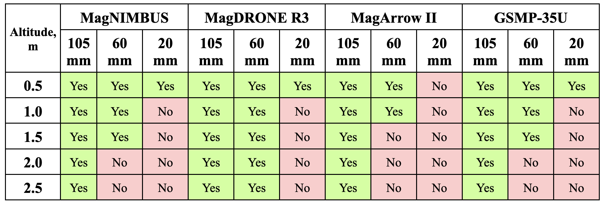
All of the above results are compiled in Table 1 for an overview. The detection confirmation is given to cases with a sufficient signal. In all other cases, there might have been a suspicion of signal being noise or no signal being present. In a real-life scenario, it would be up to the specialists to include all signals at the expense of greatly increased false positives or select only reliable signals at the risk of missing targets.
Table 1. Comparison of the detection capabilities of all the tested sensors. “Yes” means reliably detected, while “No” means not detected or unsure detection.
Flight altitude variations
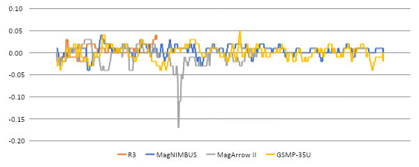
Searching for UXOs, especially small ones, based on their magnetic signals requires precise altitude keeping, as the magnetic field (and thus, the detection distance) decreases with distance as a 3rd power. Smaller UXOs barely in the detection limit can be easily undetected if the sensor does not keep a precise altitude above the ground. For example, assuming a noise floor of 10 nT, a 40-mm shell that a magnetometer can still detect at a distance of 54 centimeters would likely be undetectable if the flight altitude is raised by just 15 centimeters (reference: Billings et al. 2006, Magnetic Models of Unexploded Ordnance).
Flight altitude variation is shown in Figure 18 to address the potential concerns regarding the precision of altitude keeping for the different magnetometer setups, especially MagArrow II and GSMP-35U, which are suspended in cables 3 and 5 meters below the UAV. To ensure the magnetometers do not interfere with the TTF sensor, it was placed on a special extension off the side of the UAV (see Figures 4 and 5 in the Methods section).
Flight time
The flight times differed based on the chosen speed as recommended by the manufacturer for the test conditions, but for MagDRONE R3, it was also due to the dual-sensor setup. This allowed rapid field surveying, completing a single altitude flight in only 1.5 minutes. MagArrow II was flown at the same speed as R3 but with only one sensor thus, the flight time was 3 minutes. MagNIMBUS and GSMP-35U finished their single altitude flights at slightly more than 5 minutes.
Conclusions
- SENSYS MagDRONE R3 showed the best results of all the tested sensors, detecting the 105-mm shell at all heights and the 60-mm shell at most heights. The SPH Engineering MagNIMBUS and GEM Systems DRONEmag GSMP-35U couldn’t reliably detect the 60-mm shell at 2.0 and 2.5 meters, respectively. The Geometrics MagArrow II didn’t show a clear signal of the 60-mm shell at 1.5 m altitude and never detected the 20-mm shell.
- This test proves no benefit of using a “suspended” system like MagArrow II or GSMP-35U over a “fixed” system like MagNIMBUS or R3 at the specific survey conditions. Although noticeable, the magnetic noise of the UAV motors is less problematic than the swaying of the setup and the resulting heading error.
- UXO magnetic surveys necessitate reliable field coverage with a fixed separation distance and precise altitude keeping to increase the chance of detecting small anomalies and decreasing false positives.
Appendix - data processing steps
MagNIMBUS
Using Oasis Montaj:
1. Applied Lag Correction (fiducials):
0.5m: -50
1.0m: -140
1.5m: -130
2.0m: -140
2.5m: -140
2. Applied low-pass filter of 100 fiducials (corresponding to ~0.2 m point separation).
3. Applied Rolling Median filter of 10000 fiducials (corresponding to ~20 m distance).
4. Generated residual anomaly grid with cell size 0.2 m, color scale Histogram equalization.
5. Calculated Analytic Signal based on residual anomaly grid.
6. Applied 3x3 convolution 1 pass smoothing to the AS grid and changed the color scale to Normal distribution.
MagDRONE R3
- Using SENSYS MagDrone DataTool:
1.1. Imported file 20230920_142316_MD-R3_#0207.mdd
1.2. Divided tracks: 20deg, 1.5m.
1.3. No filters or downsampling.
1.4. Loaded GNSS RTK data.
1.5. Exported to .asc file.
- Using Oasis Montaj:
2.1. Divided flights according to their heights into separate databases.
2.2. Separated each flight in lines by sensor number.
2.3. Corrected time lag: +150 fiducials.
2.4. Applied Low Pass Filter of 25 fiducials (corresponding to ~0.2 m point separation).
2.5. Applied Rolling Median filter of 2500 fiducials (corresponding to ~20 m distance).
2.6. Generated residual anomaly grid with cell size 0.2 m and calculated Analytic Signal.
2.7. Applied 3x3 convolution 1 pass smoothing to the AS grid and changed the color scale to Normal distribution.
MagArrow II
Using Geometrics Survey Manager:
1. Data converted from MagArrow .magdata to .csv data format.
Using Oasis Montaj:
1. Imported precise GPS RTK coordinates into the magnetic data database.
2. Split data into lines according to the flight altitude.
3. Applied Heading correction with data acquired on calibration flight.
4. Applied Lag Correction of +750 fiducials.
5. Applied low-pass filter of 100 fiducials (corresponding to ~0.2 m point separation).
6. Applied Rolling Median filter of 10000 fiducials (corresponding to ~20 m window).
7. Generated residual anomaly grid with cell size 0.2 m, color scale Histogram equalization.
8. Calculated Analytic Signal.
9. Applied 3x3 convolution 1 pass smoothing to the AS grid and changed the color scale to Normal distribution.
GSMP-35U
Using Oasis Montaj:
- Imported precise GPS RTK coordinates into the magnetic data database.
- Applied Lag Corrections (fiducials):
0.5m: +15
1.0m: +15
1.5m: +7
2.0m: +7
2.5m: +7 - Applied low-pass filter of 4 fiducials (corresponding to 0.2 m separation)
- Applied Rolling Median filter of 400 fiducials (corresponding to 20 m window).
- Generated residual anomaly grid with cell size 0.2 m, color scale Histogram equalization.
- Calculated Analytic Signal based on residual anomaly grid.
- Applied 3x3 convolution 1 pass smoothing to the AS grid and changed the color scale to Normal distribution.
.jpg)